| Software | BitScope DSO | Online Demo |
 This display export shows a single frame of mixed signal data being adjusted and examined. The file that was used to create this example is called mixed.csv in the Offline Examples. For details about how to play this on your own PC, read the Sydney BitScope page. (Re)power the DSO, load this file and what you see looks nothing like this animation! This is because the (default) timebase (50ns/Div) and DSO Instrument are different. To set up DSO to display this part of the waveform as a deep capture logic image:  Timebase Zoom
What you should see on the display is the first frame of the animation above. By increasing the timebase zoom up to a value of x50 you should see the time scale expand as in the animation. You can see (by right-clicking the timebase zoom) that you can in fact expand to a factor of up to x1000 if you want, however we won't go that far just now. Next, using the waveform offset control, adjust the horizontal position of the waveform until the post-trigger delay (as reported via the TD scope variable) is 498uS.  Now click the BOTH display selector to display both the analog and logic waveforms. You can now enable the cursors and using the mouse pick up (ie, click and drag) first the POINT (RED) cursor and then the MARK (white) cursor to any features you wish to measure. You will see that the cursors apply the same way to both analog waveform and logic displays. It is therefore possible to measure times between the analog and digital (ie, logic) domains very easily. As with the post-trigger delay scope variable (TD), the cursor variables (TM and TP) report the time values at the cursor positions. Read the cursors guide for more details. Visit the next page (X-Y Plot) to learn about X-Y plots with BitScope. |
Copyright © 2023 BitScope Designs